ETC5523: Communicating with Data

From model outputs to communicative tables

Lecturer: Michael Lydeamore

Department of Econometrics and Business Statistics

michael.lydeamore@monash.edu
Week 5
cwd.numbat.space

Aim

Extract information from model objects
Select and present model results for a particular audience

Why

Model objects contain much more information than an audience needs
Good communication depends on selecting, interpreting and presenting the right results

📈 Statistical models

All models are approximations of an unknown data-generating process
Their usefulness depends on the question, the data, the assumptions and the model choice

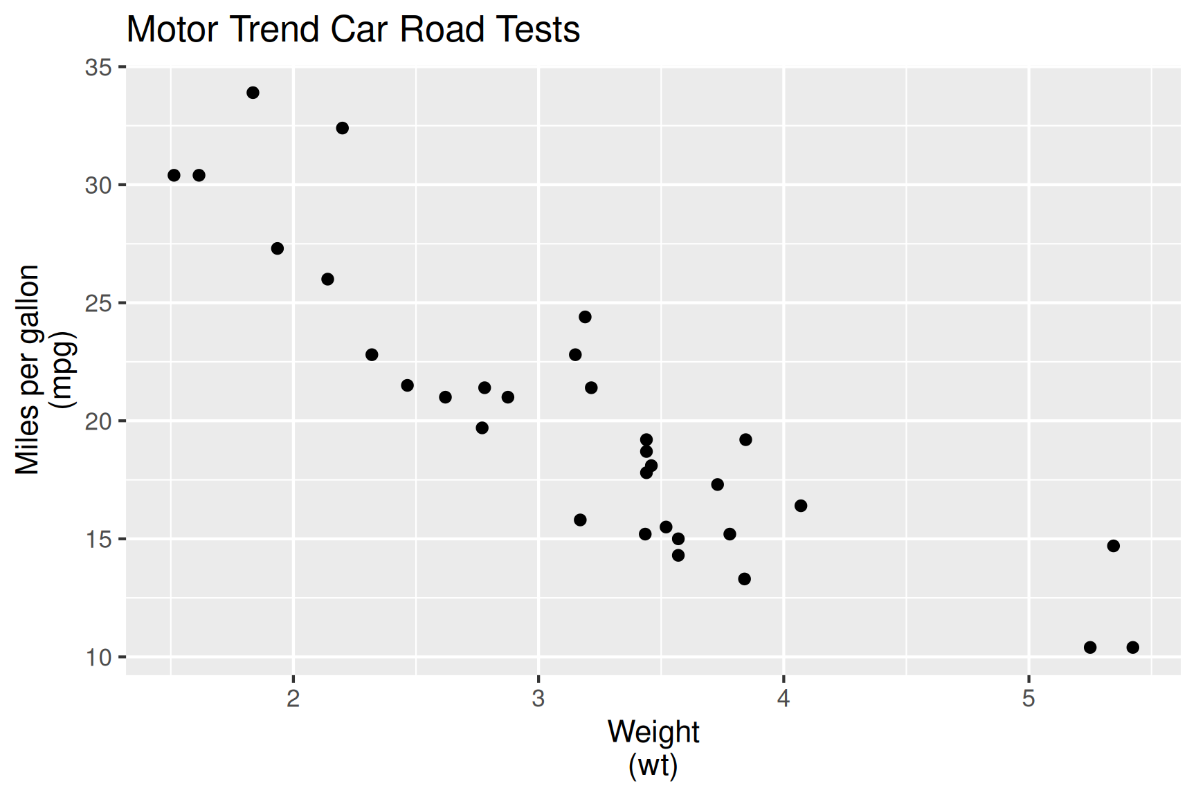
🎯 Characterise mpg in terms of wt.

Fitting linear models in R

We fit the model:

\[\texttt{mpg}_i = \beta_0 + \beta_1\texttt{wt}_i + e_i\]

In R we fit this as

fit <- lm(mpg ~ wt, data = mtcars)

\(\hat{\beta}_0 = 37.285\) and \(\hat{\beta}_1 = -5.344\)

In mtcars, wt is measured in 1,000 lb. A car that is 1,000 lb heavier is estimated to achieve 5.34 fewer mpg, on average.

ℹ️ Extracting information from the fitted model

A fitted model contains several kinds of information, including:
- the model parameter estimates,
- model-related summary statistics, e.g. \(R^2\), AIC and BIC,
- model-related values, e.g. residuals, fitted values and predictions.
So how do you extract these values from the fit?
What does fit even contain?

ℹ️ Extracting information from the fitted model

str(fit)

List of 12
 $ coefficients : Named num [1:2] 37.29 -5.34
  ..- attr(*, "names")= chr [1:2] "(Intercept)" "wt"
 $ residuals    : Named num [1:32] -2.28 -0.92 -2.09 1.3 -0.2 ...
  ..- attr(*, "names")= chr [1:32] "Mazda RX4" "Mazda RX4 Wag" "Datsun 710" "Hornet 4 Drive" ...
 $ effects      : Named num [1:32] -113.65 -29.116 -1.661 1.631 0.111 ...
  ..- attr(*, "names")= chr [1:32] "(Intercept)" "wt" "" "" ...
 $ rank         : int 2
 $ fitted.values: Named num [1:32] 23.3 21.9 24.9 20.1 18.9 ...
  ..- attr(*, "names")= chr [1:32] "Mazda RX4" "Mazda RX4 Wag" "Datsun 710" "Hornet 4 Drive" ...
 $ assign       : int [1:2] 0 1
 $ qr           :List of 5
  ..$ qr   : num [1:32, 1:2] -5.657 0.177 0.177 0.177 0.177 ...
  .. ..- attr(*, "dimnames")=List of 2
  .. .. ..$ : chr [1:32] "Mazda RX4" "Mazda RX4 Wag" "Datsun 710" "Hornet 4 Drive" ...
  .. .. ..$ : chr [1:2] "(Intercept)" "wt"
  .. ..- attr(*, "assign")= int [1:2] 0 1
  ..$ qraux: num [1:2] 1.18 1.05
  ..$ pivot: int [1:2] 1 2
  ..$ tol  : num 1e-07
  ..$ rank : int 2
  ..- attr(*, "class")= chr "qr"
 $ df.residual  : int 30
 $ xlevels      : Named list()
 $ call         : language lm(formula = mpg ~ wt, data = mtcars)
 $ terms        :Classes 'terms', 'formula'  language mpg ~ wt
  .. ..- attr(*, "variables")= language list(mpg, wt)
  .. ..- attr(*, "factors")= int [1:2, 1] 0 1
  .. .. ..- attr(*, "dimnames")=List of 2
  .. .. .. ..$ : chr [1:2] "mpg" "wt"
  .. .. .. ..$ : chr "wt"
  .. ..- attr(*, "term.labels")= chr "wt"
  .. ..- attr(*, "order")= int 1
  .. ..- attr(*, "intercept")= int 1
  .. ..- attr(*, "response")= int 1
  .. ..- attr(*, ".Environment")=<environment: R_GlobalEnv> 
  .. ..- attr(*, "predvars")= language list(mpg, wt)
  .. ..- attr(*, "dataClasses")= Named chr [1:2] "numeric" "numeric"
  .. .. ..- attr(*, "names")= chr [1:2] "mpg" "wt"
 $ model        :'data.frame':  32 obs. of  2 variables:
  ..$ mpg: num [1:32] 21 21 22.8 21.4 18.7 18.1 14.3 24.4 22.8 19.2 ...
  ..$ wt : num [1:32] 2.62 2.88 2.32 3.21 3.44 ...
  ..- attr(*, "terms")=Classes 'terms', 'formula'  language mpg ~ wt
  .. .. ..- attr(*, "variables")= language list(mpg, wt)
  .. .. ..- attr(*, "factors")= int [1:2, 1] 0 1
  .. .. .. ..- attr(*, "dimnames")=List of 2
  .. .. .. .. ..$ : chr [1:2] "mpg" "wt"
  .. .. .. .. ..$ : chr "wt"
  .. .. ..- attr(*, "term.labels")= chr "wt"
  .. .. ..- attr(*, "order")= int 1
  .. .. ..- attr(*, "intercept")= int 1
  .. .. ..- attr(*, "response")= int 1
  .. .. ..- attr(*, ".Environment")=<environment: R_GlobalEnv> 
  .. .. ..- attr(*, "predvars")= language list(mpg, wt)
  .. .. ..- attr(*, "dataClasses")= Named chr [1:2] "numeric" "numeric"
  .. .. .. ..- attr(*, "names")= chr [1:2] "mpg" "wt"
 - attr(*, "class")= chr "lm"

ℹ️ Extracting information from the fitted model

Use accessor functions to retrieve model results:

coef(fit)

(Intercept)          wt 
  37.285126   -5.344472

This gives us the estimates of \(\beta_0\) and \(\beta_1\).

An estimate is more useful when accompanied by its uncertainty:

confint(fit)

                2.5 %    97.5 %
(Intercept) 33.450500 41.119753
wt          -6.486308 -4.202635

ℹ️ Extracting information from the fitted model

You can also get a summary of the model object:

summary(fit)


Call:
lm(formula = mpg ~ wt, data = mtcars)

Residuals:
    Min      1Q  Median      3Q     Max 
-4.5432 -2.3647 -0.1252  1.4096  6.8727 

Coefficients:
            Estimate Std. Error t value Pr(>|t|)    
(Intercept)  37.2851     1.8776  19.858  < 2e-16 ***
wt           -5.3445     0.5591  -9.559 1.29e-10 ***
---
Signif. codes:  0 '***' 0.001 '**' 0.01 '*' 0.05 '.' 0.1 ' ' 1

Residual standard error: 3.046 on 30 degrees of freedom
Multiple R-squared:  0.7528,    Adjusted R-squared:  0.7446 
F-statistic: 91.38 on 1 and 30 DF,  p-value: 1.294e-10

The printed summary is useful for inspection, but it is not an audience-ready result.

Model objects to tidy data

broom::tidy(fit)

# A tibble: 2 × 5
  term        estimate std.error statistic  p.value
  <chr>          <dbl>     <dbl>     <dbl>    <dbl>
1 (Intercept)    37.3      1.88      19.9  8.24e-19
2 wt             -5.34     0.559     -9.56 1.29e-10

broom::glance(fit)

# A tibble: 1 × 12
  r.squared adj.r.squared sigma statistic  p.value    df logLik   AIC   BIC
      <dbl>         <dbl> <dbl>     <dbl>    <dbl> <dbl>  <dbl> <dbl> <dbl>
1     0.753         0.745  3.05      91.4 1.29e-10     1  -80.0  166.  170.
# ℹ 3 more variables: deviance <dbl>, df.residual <int>, nobs <int>

broom::augment(fit)

# A tibble: 32 × 9
   .rownames           mpg    wt .fitted .resid   .hat .sigma .cooksd .std.resid
   <chr>             <dbl> <dbl>   <dbl>  <dbl>  <dbl>  <dbl>   <dbl>      <dbl>
 1 Mazda RX4          21    2.62    23.3 -2.28  0.0433   3.07 1.33e-2    -0.766 
 2 Mazda RX4 Wag      21    2.88    21.9 -0.920 0.0352   3.09 1.72e-3    -0.307 
 3 Datsun 710         22.8  2.32    24.9 -2.09  0.0584   3.07 1.54e-2    -0.706 
 4 Hornet 4 Drive     21.4  3.22    20.1  1.30  0.0313   3.09 3.02e-3     0.433 
 5 Hornet Sportabout  18.7  3.44    18.9 -0.200 0.0329   3.10 7.60e-5    -0.0668
 6 Valiant            18.1  3.46    18.8 -0.693 0.0332   3.10 9.21e-4    -0.231 
 7 Duster 360         14.3  3.57    18.2 -3.91  0.0354   3.01 3.13e-2    -1.31  
 8 Merc 240D          24.4  3.19    20.2  4.16  0.0313   3.00 3.11e-2     1.39  
 9 Merc 230           22.8  3.15    20.5  2.35  0.0314   3.07 9.96e-3     0.784 
10 Merc 280           19.2  3.44    18.9  0.300 0.0329   3.10 1.71e-4     0.100 
# ℹ 22 more rows

Each `broom` verb answers a different question

Verb	Unit of output	Use it to find…
`tidy(fit)`	one row per model term	estimates, standard errors and uncertainty
`glance(fit)`	one row per model	model-level summaries such as \(R^2\), AIC and sample size
`augment(fit)`	one row per observation	fitted values, residuals and influence measures

The same interface works across many model classes. broom selects the appropriate method from the class of the fitted object.

From model object to communicative table

Extract the model terms you need

broom::tidy(fit, conf.int = TRUE)

# A tibble: 2 × 7
  term        estimate std.error statistic  p.value conf.low conf.high
  <chr>          <dbl>     <dbl>     <dbl>    <dbl>    <dbl>     <dbl>
1 (Intercept)    37.3      1.88      19.9  8.24e-19    33.5      41.1 
2 wt             -5.34     0.559     -9.56 1.29e-10    -6.49     -4.20

The tidy output is data. We can now select, rename and present the results without copying values from the printed model summary.

A default table is a starting point

default_model_table <- gtsummary::tbl_regression(
  fit,
  intercept = TRUE
)

default_model_table

The default table exposes the model output

Characteristic	Beta	95% CI	p-value
(Intercept)	37	33, 41	<0.001
wt	-5.3	-6.5, -4.2	<0.001
Abbreviation: CI = Confidence Interval

Critique the table for a general audience

Imagine this table will go to a technically competent, time-poor manager.

Which row answers the substantive question?
Can the labels be understood without seeing the R code?
Does the displayed precision match the strength of the evidence?
Is the \(p\)-value necessary for this audience?
What interpretation or limitation must accompany the table?

Refine the table for its communication purpose

model_table <- gtsummary::tbl_regression(
  fit,
  intercept = FALSE,
  label = list(wt ~ "Weight (1,000 lb)"),
  estimate_fun = gtsummary::label_style_sigfig(digits = 2)
) |>
  gtsummary::modify_column_hide(columns = p.value) |>
  gtsummary::bold_labels()

model_table

The revised table prioritises the useful result

Characteristic	Beta	95% CI
Weight (1,000 lb)	-5.3	-6.5, -4.2
Abbreviation: CI = Confidence Interval

Interpret the result before formatting it

Important

Each additional 1,000 lb of vehicle weight is associated with 5.34 fewer mpg, on average (95% confidence interval: 4.2 to 6.49 fewer mpg).

The unit of comparison is explicit.
The interval communicates uncertainty around the estimate.
“Associated with” does not claim that greater weight caused the difference.
The intercept describes a hypothetical car weighing zero and is not substantively useful here.

What results should you present?

Start with the communication question, not with everything the model produced.

Which estimate or comparison answers the audience’s question?
What uncertainty should accompany it?
What units, reference categories and sample size are needed?
Which model summary or diagnostic matters for this purpose?
What limitation prevents overinterpretation?

Tables and plots support different tasks

Use a table when readers need exact values or must look up individual results.
Use a plot when readers need to compare magnitudes, patterns or uncertainty quickly.
Use both when the tasks are genuinely different—not simply to repeat the same information.

Some common tables

Use the same workflow for descriptive summaries

summary_table <- mtcars |>
  mutate(cyl = factor(cyl)) |>
  select(mpg, wt, cyl) |>
  gtsummary::tbl_summary(
    by = cyl,
    label = list(
      mpg ~ "Fuel economy (mpg)",
      wt ~ "Weight (1,000 lb)"
    ),
    statistic = gtsummary::all_continuous() ~ "{mean} ({sd})",
    digits = gtsummary::all_continuous() ~ 1,
    missing = "no"
  ) |>
  gtsummary::bold_labels()

summary_table

A descriptive table should make comparison easy

Characteristic	4 N = 11¹	6 N = 7¹	8 N = 14¹
Fuel economy (mpg)	26.7 (4.5)	19.7 (1.5)	15.1 (2.6)
Weight (1,000 lb)	2.3 (0.6)	3.1 (0.4)	4.0 (0.8)
¹ Mean (SD)

The columns create the comparison between cylinder groups.
The labels state the measures and units.
Mean (SD) is a choice—not an automatic default. Another question or distribution may call for median (IQR).

Descriptive summary statistics

The main goal is to give a numerical summary to give a “feel” of what the data contains. These generally should convey:
- variables in the data,
- the number of observations for each variable,
- missing values (if any),
- the distribution, e.g. in the form of five-number summaries or counts/percentages for categorical variables.

Descriptive summary statistics

For numerical variables, you may have a correlation table which displays the correlation coefficients of every pair of variables. Because it is symmetrical, you can omit the upper triangle.

name	Mean	SD	1.	2.
mpg	20.09062	6.0269481
wt	3.21725	0.9784574	-0.8676594
hp	146.68750	68.5628685	-0.7761684	0.6587479

Descriptive summary statistics

options(knitr.kable.NA = '')
mtcars |>
  select(mpg, wt, hp) |>
  pivot_longer(everything()) |>
  mutate(name = factor(name, levels = c("mpg", "wt", "hp"))) |>
  group_by(name) |>
  summarise(
    Mean = mean(value),
    SD = sd(value)
  ) |>
  mutate(
    `1.` = case_when(
      name == "wt" ~ cor(mtcars$mpg, mtcars$wt),
      name == "hp" ~ cor(mtcars$mpg, mtcars$hp),
      TRUE ~ NA_real_
    ),
    `2.` = case_when(
      name == "hp" ~ cor(mtcars$wt, mtcars$hp),
      TRUE ~ NA_real_
    )
  ) |>
  knitr::kable(table.attr = "class='cor-table'") |> 
  kable_classic(full_width = FALSE)

Descriptive summary statistics

You may have cross-tabulations (also called contingency tables)

cyl/gear	3	4	5	Total
4	3.1% (1)	25.0% (8)	6.2% (2)	34.4% (11)
6	6.2% (2)	12.5% (4)	3.1% (1)	21.9% (7)
8	37.5% (12)	0.0% (0)	6.2% (2)	43.8% (14)
Total	46.9% (15)	37.5% (12)	15.6% (5)	100.0% (32)

Descriptive summary statistics

You may have cross-tabulations (also called contingency tables)

library(janitor)
mtcars |> 
  tabyl(cyl, gear) |> 
  adorn_totals(where = c("row", "col")) |> 
  adorn_percentages("all") |>
  adorn_pct_formatting(digits = 1) |>
  adorn_ns() |> 
  adorn_title("combined") |> 
  knitr::kable(table.attr = "class='xtab'") |> 
  kable_styling() |> 
  row_spec(4, extra_css = "border-top: 1px solid black;") |> 
  kable_classic(full_width = FALSE)

Model-results tables

Include the estimates or comparisons that answer the audience’s question.
Accompany estimates with a standard error, confidence interval or credible interval.
State units, reference categories and sample size where they are needed for interpretation.
Include model-level summaries such as \(R^2\), AIC or BIC only when they serve the communication purpose.
A \(p\)-value or significance stars do not replace effect size and uncertainty.

Communication considerations for tables

Numerical precision

Select an appropriate precision for your goal and audience:

	Weight
Car brand	5 d.p.	2 d.p.	0 d.p.
Mazda RX4	2.61937	2.62	3
Mazda RX4 Wag	2.87518	2.88	3
Datsun 710	2.31916	2.32	2
Hornet 4 Drive	3.21660	3.21	3

Numerical precision

Display trailing zeroes to match selected precision of the column:

Trailing zeroes
Yes	No
0.233	0.233
0.320	0.32
0.400	0.4
0.343	0.343

Numerical precision

Change and display units as appropriate:

Car brand	Weight (lb)	Weight (1,000 lb)	Weight (kg)	Weight (g)	Weight (mg)
Mazda RX4	2620	2.620	1188	1190000	1,188,000,000
Mazda RX4 Wag	2875	2.875	1304	1300000	1,304,000,000
Datsun 710	2320	2.320	1052	1050000	1,052,000,000
Hornet 4 Drive	3215	3.215	1458	1460000	1,458,000,000

Use digit-grouping conventions familiar to your audience.
For example, 1,000,000 is easier to read than 1000000 for an Australian audience.

scales::comma(c(439024, 4900343), accuracy = 1000)

[1] "439,000"   "4,900,000"

Column alignment

Centre spanner labels.
Right-align numbers.
Left-align text.

Car brand			Horsepower
Left	Center	Right	Left	Center	Right
Mazda RX4	Mazda RX4	Mazda RX4	110	110	110
Mazda RX4 Wag	Mazda RX4 Wag	Mazda RX4 Wag	110	110	110
Datsun 710	Datsun 710	Datsun 710	93	93	93
Hornet 4 Drive	Hornet 4 Drive	Hornet 4 Drive	110	110	110

Labels within tables

Tables intended as final products should use clear, descriptive labels.
Put the unit once in the column heading.
Do not repeat the unit in every cell.

❌

car	wt	disp
Mazda RX4	2620 lb	160 cubic inches
Mazda RX4 Wag	2875 lb	160 cubic inches
Datsun 710	2320 lb	108 cubic inches
Hornet 4 Drive	3215 lb	258 cubic inches
Hornet Sportabout	3440 lb	360 cubic inches
Valiant	3460 lb	225 cubic inches

Labels within tables

Tables intended as final products should use clear, descriptive labels.
Put the unit once in the column heading.
Do not repeat the unit in every cell.

✅

Car brand	Weight (1,000 lb)	Displacement (cubic inches)
Mazda RX4	2.620	160
Mazda RX4 Wag	2.875	160
Datsun 710	2.320	108
Hornet 4 Drive	3.215	258
Hornet Sportabout	3.440	360
Valiant	3.460	225

Week 5 Lesson

Summary

Use accessors and broom to turn a fitted model into data you can work with.
Select results according to the audience’s question—not simply because the model produced them.
Communicate estimates with uncertainty, units, context and appropriate limitations.
Use gtsummary to create a table, then refine its precision, alignment and labels.

Resources

ETC5523: Communicating with Data

From model outputs to communicative tables

📈 Statistical models

Fitting linear models in R

ℹ️ Extracting information from the fitted model

ℹ️ Extracting information from the fitted model

ℹ️ Extracting information from the fitted model

ℹ️ Extracting information from the fitted model

Model objects to tidy data

Each broom verb answers a different question

From model object to communicative table

Extract the model terms you need

A default table is a starting point

The default table exposes the model output

Critique the table for a general audience

Refine the table for its communication purpose

The revised table prioritises the useful result

Interpret the result before formatting it

What results should you present?

Tables and plots support different tasks

Some common tables

Use the same workflow for descriptive summaries

A descriptive table should make comparison easy

Descriptive summary statistics

Descriptive summary statistics

Descriptive summary statistics

Descriptive summary statistics

Descriptive summary statistics

Model-results tables

Communication considerations for tables

Numerical precision

Numerical precision

Numerical precision

Column alignment

Labels within tables

Labels within tables

Week 5 Lesson

Each `broom` verb answers a different question