ETC5523: Communicating with Data
Tutorial 5
🎯 Objectives
- create new functions and generic methods
- understand and follow guidelines for best way to communicate with tables
- construct regression, descriptive, and interactive tables with R Markdown
- deconstruct and manipulate “novel” model objects
- modify the look of HTML tables produced by R Markdown or Quarto
Preparation
Install the R-packages
install.packages(c("broom", "DT", "kableExtra", "palmerpenguins", "modelsummary", "gtsummary"))👥 Exercise 5A
Reporting regression tables
Create regression tables, respecting the standard guidelines of presentation for tables, with models lm1 and rlm1 below using modelsummary, gtsummary or otherwise.
🛠️ Exercise 5B
Interactive data tables
Produce the same table that you find below using DT using the penguins data in the palmerpenguins package.
👥 Exercise 5C - Challenge
Working with robust linear models
Consider the artificial data in the object df. There are two obvious outliers. Which observations are the outliers?
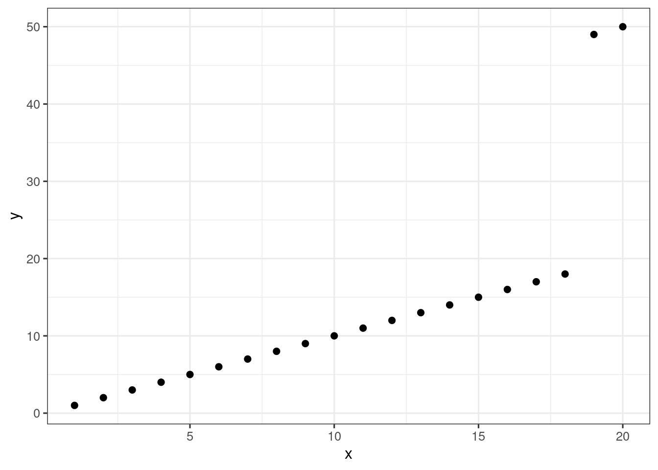
A simple linear model where parameters are estimated using least squares estimate are not robust to outliers. Below we fit two models:
- a linear model with least square estimates contained in
fit_lmand - a robust linear model contained in
fit_rlm.
To explain briefly, a robust linear model down-weights the contribution of the observations that are outlying observations to estimate parameters.
fit_lm <- lm(y ~ x, data = df)
fit_rlm <- rlm(y ~ x, data = df)
Below is a modification to the augment method from the broom package to extract some model-related values and the weights from the iterated re-weighted least squares.
augment.rlm <- function(fit, ...) {
   broom:::augment.rlm(fit) %>%
    mutate(w = fit$w)
}

augment(fit_rlm)
# A tibble: 20 × 9
y x .fitted .resid .hat .sigma .cooksd .std.resid w
<int> <int> <dbl> <dbl> <dbl> <dbl> <dbl> <dbl> <dbl>
1 1 1 0.999 0.000546 0.206 10.3 NA NA 1
2 2 2 2.00 0.000452 0.172 10.3 NA NA 1
3 3 3 3.00 0.000358 0.143 10.3 NA NA 1
4 4 4 4.00 0.000263 0.118 10.3 NA NA 1
5 5 5 5.00 0.000169 0.0974 10.3 NA NA 1
6 6 6 6.00 0.0000749 0.0808 10.3 NA NA 1
7 7 7 7.00 -0.0000193 0.0685 10.3 NA NA 1
8 8 8 8.00 -0.000114 0.0603 10.3 NA NA 1
9 9 9 9.00 -0.000208 0.0564 10.3 NA NA 1
10 10 10 10.0 -0.000302 0.0566 10.3 NA NA 1
11 11 11 11.0 -0.000396 0.0611 10.3 NA NA 1
12 12 12 12.0 -0.000490 0.0698 10.3 NA NA 1
13 13 13 13.0 -0.000585 0.0827 10.3 NA NA 1
14 14 14 14.0 -0.000679 0.0998 10.3 NA NA 1
15 15 15 15.0 -0.000773 0.121 10.3 NA NA 1
16 16 16 16.0 -0.000867 0.147 10.3 NA NA 1
17 17 17 17.0 -0.000961 0.172 10.3 NA NA 0.977
18 18 18 18.0 -0.00106 0.187 10.3 NA NA 0.890
19 49 19 19.0 30.0 0.0000184 7.28 NA NA 0.0000742
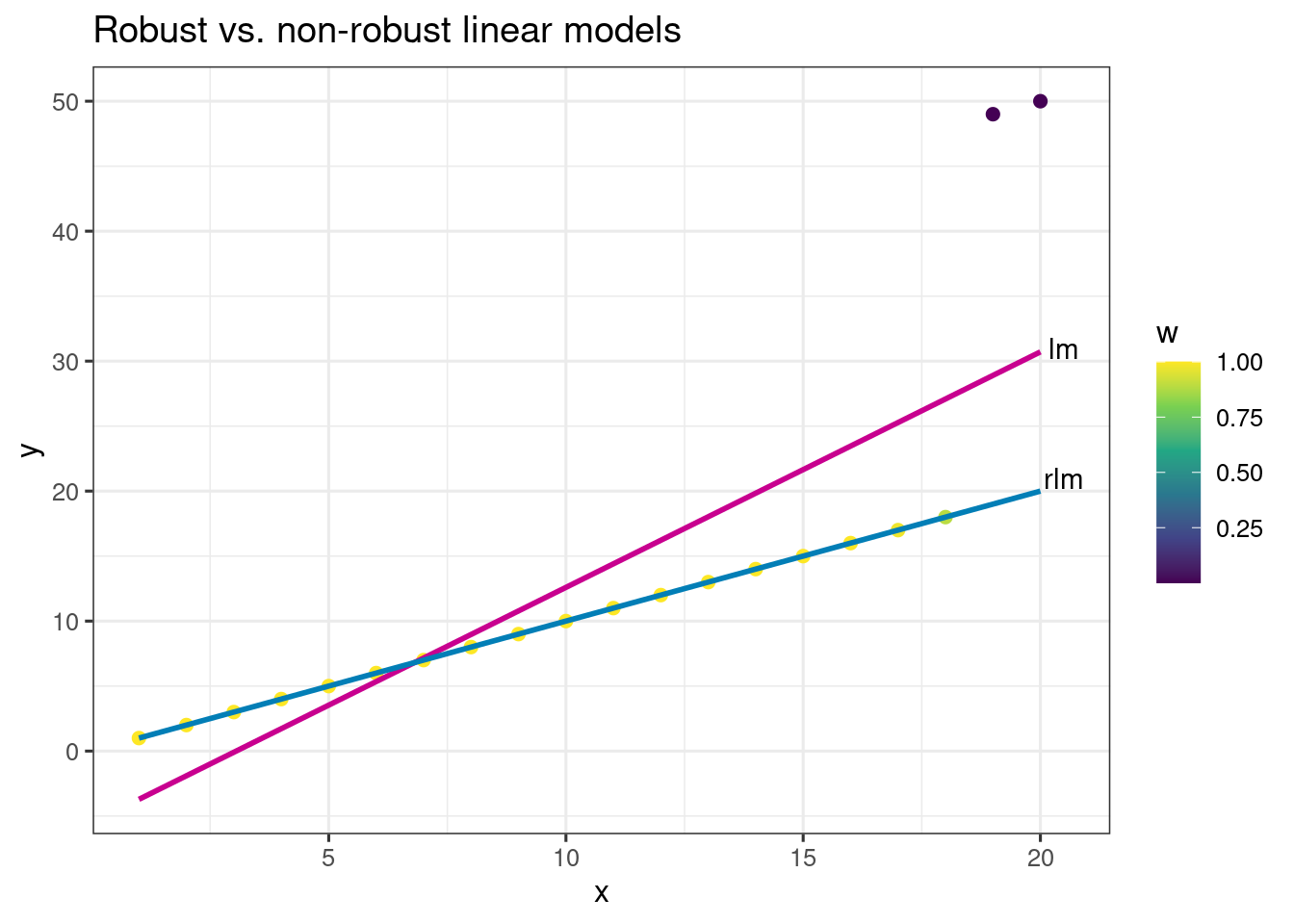
20 50 20 20.0 30.0 0.0000216 7.28 NA NA 0.0000742Here is a plot to compare the two model fits, and to give some understanding of these weights. What do you notice about the weights?
Can you
- recreate this plot using the functions in this question and
- improve the plot to better undertstand the differences in the model and the weights?